Numerical simulation of actin cortex growth.

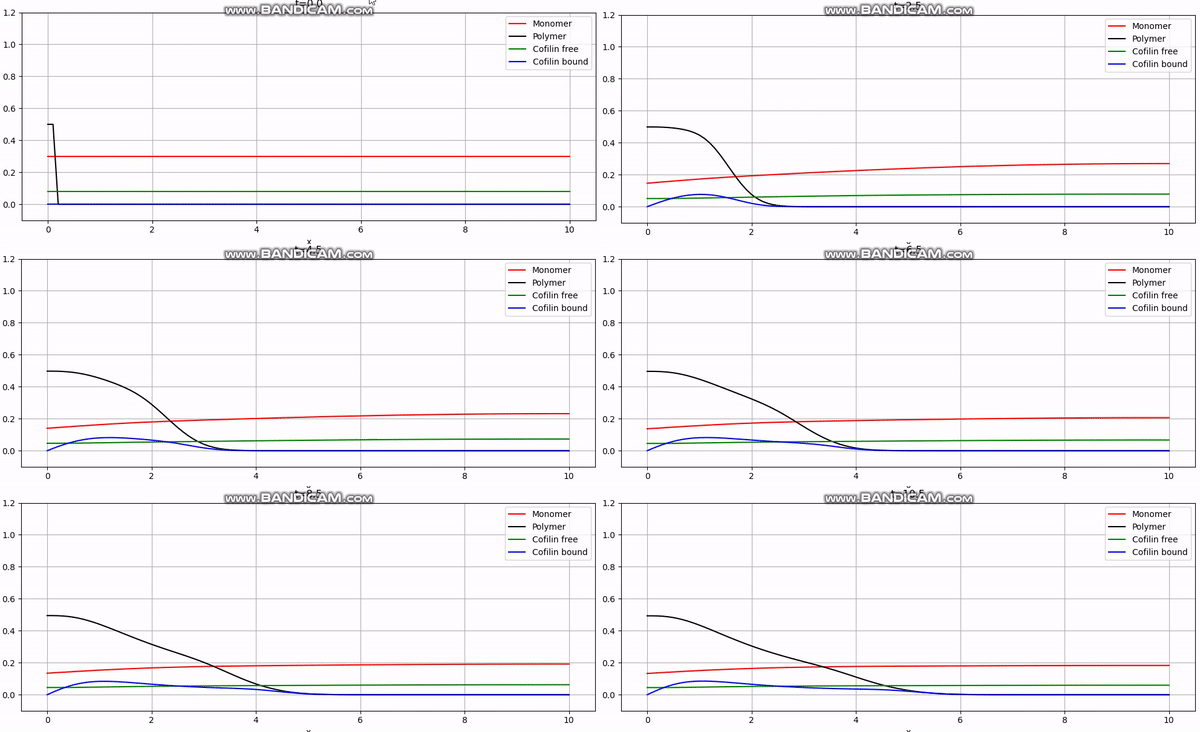
During my senior year in physics, I worked on a project that aimed to model the dynamics of a certain part of the cell called the actin cortex. The actin cortex is a thin layer of actin filaments that lies beneath the plasma membrane of eukaryotic cells. It plays a crucial role in cell mechanics, cell division, and cell motility. I validated a model supervised by my advisor and their colleagues, mainly using numerical methods (and ensuring mathematical consistency). Finally, I implemented it all in Python to obtain solutions like this:

Discretization

The model consists of a set of partial differential equations that capture the dynamics of actin monomers, filaments, and associated proteins. The complex dynamics of all these eventually create an actin cortex and maintain it in an equilibrium state. I will focus only on the discretization here, but the full model can be seen here.

To solve the model equations numerically, I used a finite difference method that discretizes the spatial domain into a grid of points and approximates the derivatives using central differences. Then, I incorporated the boundary conditions - which were quite complex.

The discretized equations:

\begin{equation} \begin{aligned} p_i^{n+1} =& p_i - \frac{\Delta t}{\Delta x} \cdot v (p_{i} - p_{i-1}) \\ &- Depoly \end{aligned} \end{equation}

\begin{equation} \begin{aligned} m_i^{n+1} =& m_i + D_m \frac{\Delta t}{2 \Delta x^2} \\ &\big[(2 - \beta (p_i + p_{i+1}))(m_{i+1}-m_i) \quad \\ &- (2 - \beta (p_i + p_{i-1}))(m_{i}-m_{i-1}) \big] \\ &+ Depoly \end{aligned} \end{equation}

\begin{equation} \begin{aligned} c_{f,i}^{n+1} &= c_{f, i} + D_c \frac{\Delta t}{\Delta x^2} \times \\ &(c_{f, i+1} + c_{f, i-1} - 2 c_{f, i}) \\ &- Bind + Depoly \end{aligned} \end{equation}

\begin{equation} \begin{aligned} c_{b,i}^{n+1} &= c_{b, i} - v \frac{\Delta t}{\Delta x} (c_{b, i} - c_{b, i-1}) \\ &+ Bind - Depoly \end{aligned} \\ \end{equation}

Where:

\begin{align} Depoly &= \Delta t \, \alpha c_{b, i} p_i \\ Bind &= \Delta t \, k_s c_{f, i} p_i \end{align}

Most of the boundary conditions were quite normal, except for one. The boundary condition for $m$ accounts for a significant part of the dynamics, namely, the polymerization (synthesis of $p$ ) on the edge. It required special treatment and turned out to be:

\begin{equation} \begin{aligned} m_0^{n+1} =& m_0 + D_m \frac{\Delta t}{2 \Delta x^2} \ \\ &\big[(2 - \beta (p_0 + p_{1}))(m_{1}-m_0) \\ &- (2 - \beta (p_0 + p_{-1}))(m_{0}-m_{-1}) \big] \end{aligned} \end{equation}

With $p_{-1}=p_{0}$ .

Implementation

Here I will present code snippets of the Python Implementation. The full code can be found here.

First, the calculation of $f$ , which includes all the $non-flux$ $terms$ in equations (1-4):

def get_f(self):
    """Calculates the f part of the discretizied equations

    Returns:
        tuple: f_p[-1:1], f_m[-1:1], f_cf[-1:1], f_cb[-1:1]
    """
    dt, dx, p, cf, cb, v = (
        self._dt,
        self._dx,
        self._p,
        self._cf,
        self._cb,
        self._v,
    )
    k_s = self._params["k_s"]
    alpha = self._alpha if isinstance(self._alpha, (int, float)) else self._alpha

    depoly = (dt * alpha) * cb * p
    bind = (dt * k_s) * cf * p

    p_prev = np.roll(p, 1)
    cb_prev = np.roll(cb, 1)

    f_p = -v * dt / (dx) * (p - p_prev) - depoly  
    f_m = depoly                                  
    f_cf = depoly - bind                          
    f_cb = -v * dt / (dx) * (cb - cb_prev) - f_cf

    return f_p, f_m, f_cf, f_cb

Now that we have a function calculating the non-flux terms, we can proceed to iterate and solve the system. Note, for instance, that under the comment ‘Calculate inner-points’ below, we explicitly implement equation (2).

def iterate_values(self):
    ...

    self._v = a_br * k_br * (m[0] ** 2) + a_gr * k_gr * (m[0] - m_c)
    v = self._v
    f = self.get_f()

    # Calculate boundaries
    p_L, m_L, cf_L, cb_L = 0, m[-3], cf[-3], 0
    p_0, cf_0, cb_0 = p[1], cf[2], 0
    m_minus_1 = m[1] - 2*dx/(Dm*(1-beta*p[0])) * p[0] * v
    m_0 = m[0] + Dm*dt/(2*dx**2) * \
                ((2-beta*(p[0] + p[1]))*(m[1] - m[0]) - (2-2*beta*p[0])*(m[0] - m_minus_1))

    # Calculate inner-points
    m_flux = Dm * dt / (2 * dx**2) * \
        (
            (2 - beta * (p[1:-1] + p[2:])) * (m[2:] - m[1:-1])
            - (2 - beta * (p[1:-1] + p[:-2])) * (m[1:-1] - m[:-2])
        )
    
    cf_flux = Dc * dt / (dx**2) * (cf[2:] + cf[:-2] - 2 * cf[1:-1])

    # Set boundaries
    p[-1], m[-1], cf[-1], cb[-1] = p_L, m_L, cf_L, cb_L
    p[0], m[0], cf[0], cb[0] = p_0, m_0, cf_0, cb_0

    # Assign new values
    p[1:-1] = p[1:-1] + f[0][1:-1]
    m[1:-1] = m[1:-1] + m_flux + f[1][1:-1]
    cf[1:-1] = cf[1:-1] + cf_flux + f[2][1:-1]
    cb[1:-1] = cb[1:-1] + f[3][1:-1]

    return p, m, cf, cb, v

The two functions above actually do the needed calculations. Now all that’s left is wrapping them in a solver!

def solver(self, live_plot=True):
    ...
    for n in t:
        err1, err2 = self.mass_sum()

        if self.user_action:
            self.user_action(
                p=p, m=m, cf=cf, cb=cb, v=v, dx=dx, dt=dt, x=x, t=t, n=n
            )

        if (
            self.validation
        ):  # Raise an error when either the monomer or cofilin deveation rise above 5%
            if abs(err1) > 5 or abs(err2) > 5:
                raise DeviationTooHighError

        if live_plot and n % self.plot_interval < 0.1 * dt:
            self.live_plot(n)

        self.iterate_values()

    if self.completion_run: # Option to run simulation until tolerance is met
            ...
            checks = [
                all(np.abs(p - p_p) < tolerance),
                all(np.abs(m - m_p) < tolerance),
                all(np.abs(cf - cf_p) < tolerance),
                all(np.abs(cb - cb_p) < tolerance),
            ]
            completed = all(checks)
            ...
    
    self.final_plot(t[-1])
    return p, m, cf, cb, x, t

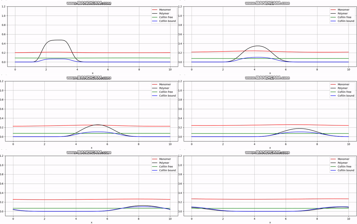
And that concludes our implementation. With additional plotting code, we achieve animations like the one above or the periodic boundary condition shown below: