Recently, at Imperial, I took a module about basic Fluid Dynamics (from a mathematical perspective). Our lecturer showed that under certain conditions, 2D fluid flow can be described fully using a complex function called “stream function”. Then, in an assignment, there was a bonus question about researching a particular type of flow (quadruple flow). We could carry out the research however we’d like, so I thought about trying to visualize it using Python and Manim (3Blue1Brown package). The result was so beautiful that I just had to share it!

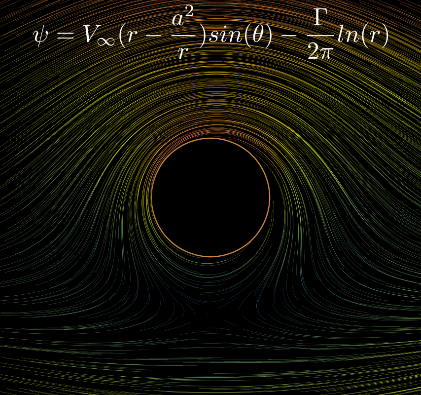
As an example, you can see the following fluid flow for a fluid going in constant motion around a circle. Imagine that the circle is spinning with some angular velocity $\Gamma$. Then our stream function $\psi(r, \theta)$, described using polar coordinates $r, \theta$, can be written as follows:

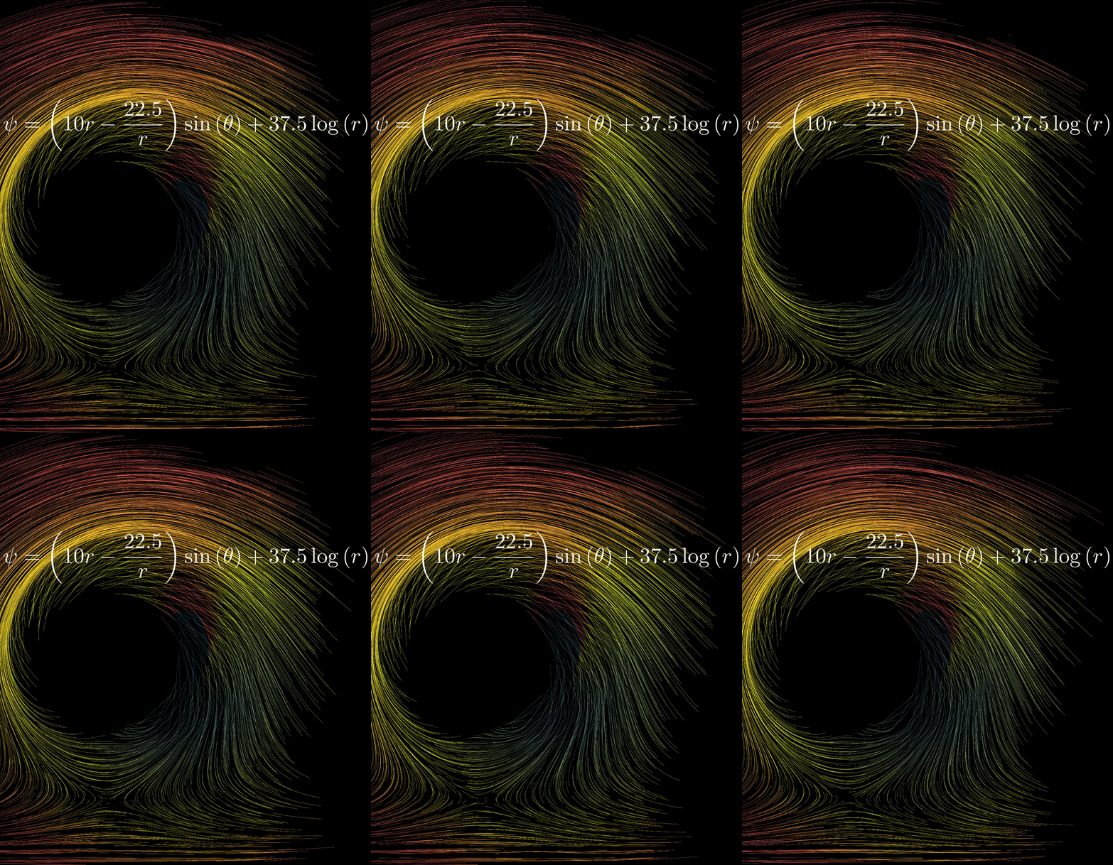
For it, we find the following flow (here $\Gamma$ is big, imagine that the circle is rotating quickly!):

Calculating Cartesian Velocity from Stream Function

To visualize the flow, we need to derive the Cartesian velocity components $u(x,y), v(x,y)$ from the stream function $\psi(r, \theta)$ (we need that because Manim takes in Cartesian coordinates). Doing this by hand can be terrible; it involves replacing $r, \theta$ with $x^2 + y^2, \text{atan}(y/x)$ respectively, and then differentiating with respect to x and y! A messy an unpleasent calculation. The good news is that we can do it using sympy!

import sympy
from manim import *


class StreamFunction:
    def __init__(self, expression, coord):
        self.expression = expression
        self.x, self.y = sympy.symbols('x y')
        
        r = self.x**2 + self.y**2
        theta = sympy.atan2(self.y, self.x)
        
        psi_cylindrical = expression.subs({coord[0]: r, coord[1]: theta})
        self.psi_cartesian = psi_cylindrical.simplify()

    def get_velocity_components(self):
        x, y = self.x, self.y
         
        u = sympy.lambdify([x, y], self.psi_cartesian.diff(y), 'numpy')
        v = sympy.lambdify([x, y], -self.psi_cartesian.diff(x), 'numpy')

        return u, v

Here, StreamFunction takes a Sympy expression of $\psi$ in polar coordinates, which is then supplied in coord. An example instance is as follows:

if __name__ == "__main__":
    a = 1.5
    v_inf = 10
    q = 5
    gamma = - 1 * sympy.pi * a * v_inf

    r, theta = sympy.symbols("r theta")    
    psi_expr = v_inf * (r - a**2/r) * sympy.sin(theta) - gamma/(2*sympy.pi) * sympy.ln(r)

    stream_function = StreamFunction(psi_expr, [r, theta])

Then, calling get_velocity_components() gives us lambda functions of $u(x,y), v(x,y)$ like we wanted! Isn’t Sympy and the lambdify method amazing?

Animating using Manim

The 3b1b package Manim can be a bit tough to learn, but you just can’t resist those beautiful math animations. In order to render the streamlines, we’ll use the StreamLines class that was written just for that. I won’t go into how to use the Manim library; you can find some good introductory articles in their documentation.

For our purposes, we’ll use this code:

class Streamlines(Scene):
    def __init__(self, stream_function, animation=False, **kwargs):
        super().__init__(**kwargs)
        self.stream_function = stream_function
        self.animation = animation

    def construct(self):
        u, v = self.stream_function.get_velocity_components()
        
        def velocity_field(pos):
            
            if pos[0]**2 + pos[1]**2 - 0.8 < 0:
                return np.array([0, 0, 0]) # Creating a black hole in the center
            
            return np.array([u(pos[0], pos[1]), v(pos[0], pos[1]), 0])
        
        contour_length = 0.8 if self.animation else 0.02

        stream_lines = StreamLines(velocity_field, virtual_time=contour_length, dt=0.01,
                                   x_range=[-2, 2, 0.1], y_range=[-2, 2, 0.1],
                                   min_color_scheme_value=20, max_color_scheme_value=130).scale(3)

        psi_latex = f"\psi = {sympy.latex(stream_function.expression)}"
        psi_label = MathTex(psi_latex, font_size=80)
        psi_label.align_on_border(UP)
        self.add(psi_label)


        if self.animation:
            self.add(stream_lines)
            stream_lines.start_animation(warm_up=False, flow_speed=0.4)
            self.bring_to_front(psi_label)

            self.wait(4)
        
        else:
            self.add(stream_lines)
            self.bring_to_front(psi_label)

In here, note that we first initialize a StreamFunction instance, then get its Cartesian velocity components u, v, and use them to define the velocity_field, which is in mathematical notation $\vec{V}(x,y)$. The velocity field also has a “black hole” in the middle because we don’t want to calculate stuff for $r=0$! Also, it helps to visualize the physics that we work with, that there is a rotating circle in the center of a uniformly flowing field.

That’s it! I hope you’ll play around with it and create some awesome fluid animations! In the meantime, here are some of mine:

Here the “disc” at the center is rotating incredibly fast (large $\Gamma$):

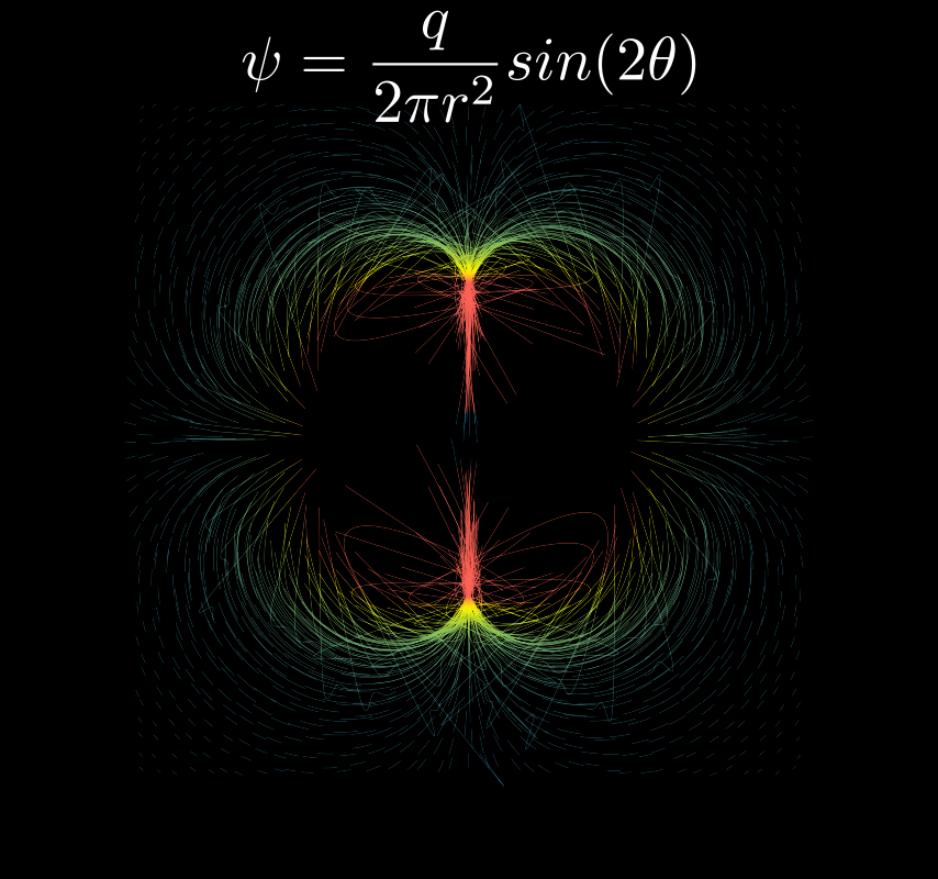
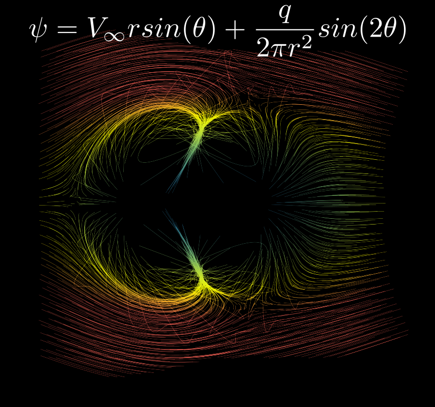
Here I tried to simulate a quadruple, and then a quadruple in uniform motion (the actual research bonus from the original assignment):