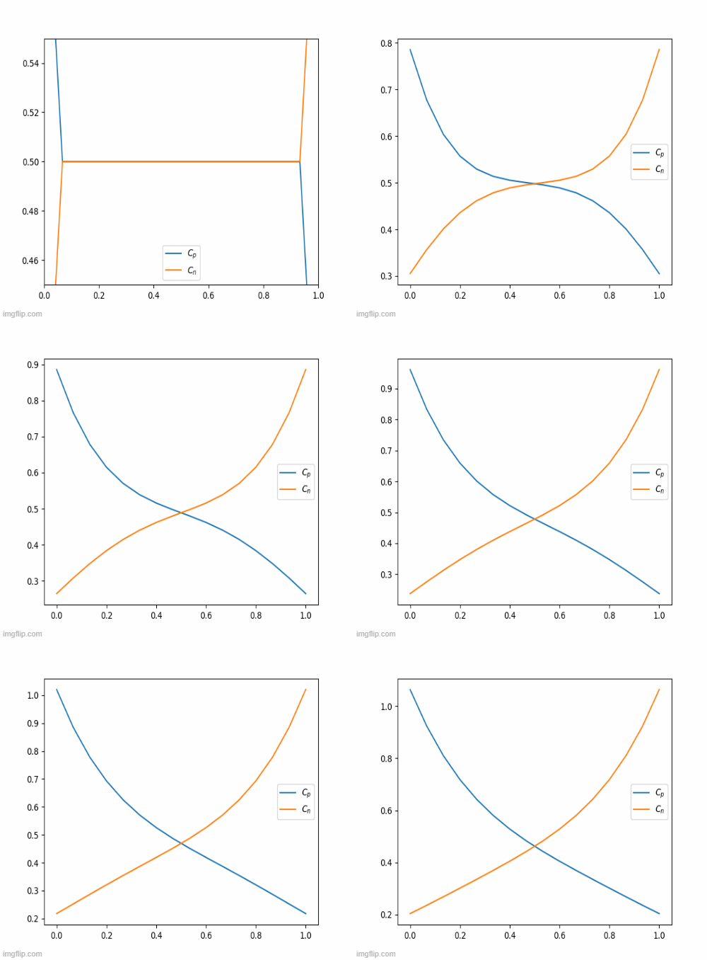
Capturing a the dynamics of a battery, with mathematics.
In one of my two undergrad senior year research projects, I present a mean-field model of the nickel-hydroxide (Ni(OH)2) electrode in the Edison rechargeable battery. The model aims to describe the electrode’s dynamics, charge transport, and phase separation. The Poisson-Nernst-Planck equation is used to describe the charge transport, while the Cahn-Hilliard approach is used to model the phase separation. Then, the model equations are solved numerically. Before presenting the project, let’s first discuss an important permilmeniry work I conducted.
Numerically Solving the PNP Equations
While my advisor and I were working on the mathematical model, I also tried to tackle my first numerical problem - solving the Poission Nernst Planck equations. I provided quite a detailed solution, which I will present here.
We would like to solve the following equations (in 1D):
Subject to the boundary conditions:
To find for all at the current step, I will use the implicit finite difference method. After applying finite difference, the potential at the point would be:
Therefore, solving for at a certain time would mean solving the following matrix:
Notice that the LHS matrix is composed of ones, and elements on each diagonal.
In python, it looks like this:
def get_phi(phi_0, phi_M, n, p, dx, n_l=0, n_r=0):
    # TODO: add phi_neumann conditions

    # Creating the coeff matrix
    coeff_matrix = np.diag(np.ones(M-2)) + np.diag(-0.5*np.ones(M-3), 1) + np.diag(-0.5*np.ones(M-3), -1)

    # Creating the RHS result vector
    result_vector = np.array([p[m]-n[m] for m in range(2, M-2)])
    right_res = p[M-2] - n[M-2] + phi_M/(dx**2)
    left_res = p[1] - n[1] + phi_0/(dx**2)
    result_vector = ((dx**2)/2)*np.append(np.insert(result_vector, 0, left_res), right_res)

    # Solving for phi and adding the boundry
    phi_trimmed = np.linalg.solve(coeff_matrix, result_vector)
    phi = np.append(np.insert(phi_trimmed, 0, phi_0), phi_M)

    return phi
Together with finding , we need to iterate . This involves finding for each . We assume that we have for every . I will use explicit central difference method to get:
This can be implemented nicely using NumPy:
def iterate_concentration(c, phi, dx, dt, positive, flux_l=0, flux_r=0, neumann=False):
    """
    Assume c and phi are 1XM vectors
    c_pp - c-prime-prime, cp - c-prime, phi_pp - phi-prime-prime, phi_p - phi-prime

    """
    sign = 1 if positive else -1

    c_1, c_M = c[0], c[M-1]
    phi_1, phi_M = phi[0], phi[M-1]
    # c_prev_1, c_prev_M = c_prev[0], c_prev[M-1]


    c_rolled = np.roll(c, 1)
    c_rolled_back = np.roll(c, -1)
    np.put(c_rolled, [0, -1], [c_1, c_M]) # Creating c_{m+1}
    np.put(c_rolled_back, [0, -1], [c_1, c_M]) # Creating c_{m-1}

    phi_rolled = np.roll(phi, 1)
    phi_rolled_back = np.roll(phi, -1)
    np.put(phi_rolled, [0, -1], [phi_1, phi_M]) # Creating phi_{m+1}
    np.put(phi_rolled_back, [0, -1], [phi_1, phi_M]) # Creating phi_{m+1}

    c_pp = c_rolled + c_rolled_back - 2*c
    c_p = c_rolled - c_rolled_back

    phi_pp = phi_rolled + phi_rolled_back - 2*phi
    phi_p = phi_rolled - phi_rolled_back
    # print(phi_p, phi_pp)

    c_iter = c + dt/(dx**2)*(c_pp + (1/4)*sign*c_p*phi_p + sign*c*phi_pp)

    if neumann:
        c_iter[0] = (dx*flux_l - c_iter[1])/(sign*(phi[1]-phi[0])-1)
        c_iter[-1] = c_iter[-2] - sign*c_iter[-2]*(phi[-1]-phi[-2]) + dx*flux_r


    return c_iter
This eventually, results in this beautiful animation

Nickel-Hydroxide Project
We started from a different set of mathematical equations, but quickly realized that we have to modify the mathematical model to our specific setup. Eventually, the model equations took the following form:
Essentialy, the equations describe the motion of the ions inside the solution, affected by diffusion, electric forces, and concentration gradients. A full description of the model, its parameters, and the code, can be found in my GitHub.
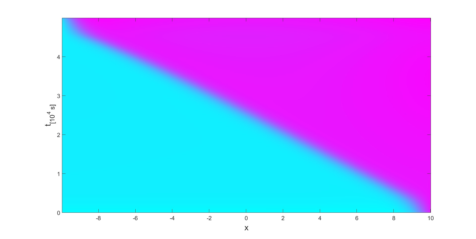
An essential part of the dynamics is the phase-transition the material undergoes (modeled with Cahn-Hilliard equations). We can observe this dynamic process in action in the following figure:

The figure was created in MatLab and it shows a Space-time plot with an input electron flux (to the electrode) from the right. The different phases are Purple - , Blue - . Over time, the phase takes over the material and the interface moves to the left edge.
After submitting the project and continuing with my studies, my advisor informed me that he and his colleagues further developed my work into a 2D model, achieving the exact behavior they sought. I hope to continue supporting their efforts and contribute to their research, aiming to publish preliminary results in the upcoming couple of years.